First Part of Even Semester

For the first meeting, I've learned about LINKED LIST. So what is linked list? Linked list is a dynamic data structure, where each element is a separate object. If in array we can easily access the elements in it by the index--because it stores the value in a consecutive memory location, in linked list we can’t do that because in linked list it uses random memory location. Now if you think “Then, isn't array better than?” well in array you can’t easily do insertions and deletions, but in linked list you can easily do push(for insertion) or pop(for deletion). Other than that, if in array you have to give a fixed memory to use in your program, in linked list the number of nodes is not fixed and can grow or shrink on demand, hence it’s called a dynamic data structure. This feature is very useful when you have to deal with an unknown number of objects. One of the disadvantage of linked list is that it uses more memory compares with an array, it adds an extra 4 bytes (on 32-bit CPU) to store a reference to the next node.       

            I have mentioned nodes before, so, what is it? In linked list we usually call each element in it as a node. A node has two things in it, a value, and a reference to the next node. The last node has a reference to NULL. The first node of a linked list is usually called the head of the list and the last node is called the tail of the list. If the list is empty then the head is a NULL reference.

            There are several types of linked list, the first one is a single linked list which was described above and the second one is a double linked list. A double linked list has the same meaning as a single linked list, just that it has an addition of a reference to the previous node too. There is also a circular linked list which has no head or tail because the tail is connected to the head. Another one is multilinked list, it has multiple additional lists from a certain mode.

Single Linked List

Double Linked List

Circular Linked List

So now I’m going to give an example on how to do the operations.

1.      Insert nodes.

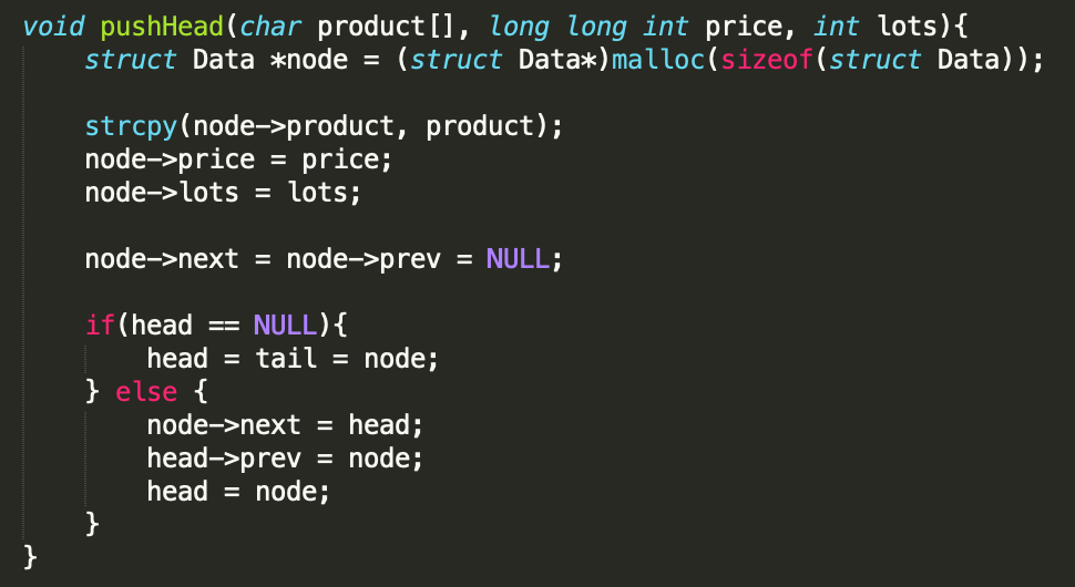
To insert a new node we can do pushHead or pushTail or pushMid.

Firstly, we will need to create a structure that defines a node. This will need to include at least one variable for data and one pointer to refer to the next node.

•  pushHead

When adding a node to the start of the list we need to take care of the following things:

a.   If the node to be added is the first node in the list then the Tail node and Head node will be the same. 

b.   If a node to be added to the list is not the first node then we need to store the head node in a temporary variable and set the Head node to the newly added node and update its next pointer to the temporary node (that was the Head node initially). In this way our newly added node becomes the Head node and it starts pointing to the older Head node that has become the second node in the list.

• pushTail

This method is used to add the node at the end of the list. It is similar to the pushHead method except we update the Tail node here instead of Head Node. 

1. If there is no node in the list then the Head node and Tail node will be the same. 
2. If we have one or more nodes then we will store the Tail node in some temporary variable and set the Tail node to the newly added node and we will update the next pointer of our temporary node to the Tail node.

• pushMid

This method is used to add the node in the middle of the list. It is just a combination of pushHead and pushTail with an addition of another function.

 2.  Remove nodes.

To remove a node we con do popHead or popTail or popMid.

• popHead 

For removing the first element in the list we must have the following points in mind:

a.   List count should not be zero. 

b.   If there is only one element in the list then the Head and Tail node must be set to null or we can also call the Clear method since there is no element in the list. 

c.   If there is more than one node in the list then we need to set the Head node to the next pointer of the Head node (that is the second node). By doing that the second element in the list becomes the Head node.

• popTail

For removing the last element in the list we must check the following:

a.   List count should not be zero. 

b.   If there is only one element in the list then the Head and Tail nodes must be set to null or we can also call the Clear method since there is no element in the list. 

c.   If there is more than one node in the list then we need to iterate among all the nodes and need to retain the previous node (because this node is going to become the Tail node). While iterating among all the nodes we need to find the node whose next pointer is null because that node is the Tail node. Since we are also maintaining the previous node we will also change its next pointer to null and set the Tail node to the previous node.

 3. View all.

To view all nodes that we have input we can make a function.

That’s all for today’s topic, I hope we all learn new things. 

From my last post, I’ve talked about single linked list and double linked list, now we’re going to talk about STACK AND QUEUE. Both stack and queue is a linear data structure. Queues and stacks are also complementary in the actual use scenarios.

So what is the difference between stack and queue? 

In STACK the elements can be inserted and deleted only from one side of the list called the TOP and a stack follows the LIFO (Last In, First Out) principle, so the element inserted at the last is the first element to come out. In stack if you want to add a new node you can do push like in a single linked list and do pop if you want to remove a node. But remember that the added new node will be put on top or say at the end of the list and if you do pop or remove a node the one that will be removed will be the top or the recently added node. One of the applications for stack is an undo mechanism in a text editor.

Here is a visualization of stack.

For QUEUE the elements can be inserted only from one side of the list called REAR(the last inserted element), and the elements can be deleted only from the other side called the FRONT(the first and still element of the list) and a queue follows the FIFO (First In, First Out) principles, so the elements inserted at first in the list will be the first to be removed from the list. In queue adding a new node--to the end of the list is called enqueue and removing the front node is called dequeue. Queue will be very useful when doing parsing or converting arithmetic expressions from infix to postfix.

Here is a visualization of queue.

That’s it for my brief summary for stack and queue, I hope we all learn something from this. 

In this post, we will talk about TREE AND HASH in Data Structure. If you have learned about linked lists, queues, and stacks, we know that those data structures are called "linear" data structures because they all have a logical start and a logical end. However, tree and hash is not a "linear" data structure. 

TREE

A tree is a collection of nodes connected by directed (or undirected) edges. A tree stored its data in a hierarchy way. The easiest way to imagine it is by using a family tree. A tree can be empty with no nodes or a tree is a structure consisting of one node called the root and zero or one or more subtrees. 

A tree has the following general properties:

• One node is distinguished as a root.
• Every node (exclude a root) is connected by a directed edge from exactly one other node; A direction is: parent -> children 

Terminology summary

Root is the topmost node of the tree

·      Edge is the link between two nodes

·      Child is a node that has a parent node

·      Parent is a node that has an edge to a child node

·      Leaf is a node that does not have a child node in the tree

·      Height is the length of the longest path to a leaf

·      Depth is the length of the path to its root

Binary Trees

A binary tree is a tree data structure in which each node has at the most two children, which are referred to as the left child and the right child. A tree is represented by a pointer to the topmost node in tree. If the tree is empty, then the value of root is NULL. A Binary Tree node contains following parts:

1.     Data

2.     Pointer to left child

3.     Pointer to right child

A Binary Tree can be traversed in two ways:

1.     Depth First Traversal: 

·    In a preorder transversal, we visit any given node before we visit its children

·    In a postorder traversal, we visit each node only after we visit its children (and their subtrees).

·    In a inorder traversal, we first visit the left child (including its enitre subtree), the visit the parent node and finally visit the right child (including its entire subtree).

2.     Breadth-First Traversal: Level Order Traversal

There are three different types of binary trees that will be discussed in this lesson:

1.       Full binary tree: Every node other than leaf nodes has 2 child nodes.

2.       Complete binary tree: All levels are filled except possibly the last one, and all nodes are filled in as far left as possible.

3.       Perfect binary tree: All nodes have two children and all leaves are at the same level.

Binary Search Tree

In Binary Search Tree is a Binary Tree with following additional properties:

·      The left subtree of a node contains only nodes with keys less than the node’s key.

·      The right subtree of a node contains only nodes with keys greater than the node’s key.

·      The left and right subtree each must also be a binary search tree.

Binary Heap

A Binary Heap is a Binary Tree with following properties.

1.     It’s a complete tree (All levels are completely filled except possibly the last level and the last level has all keys as left as possible). This property of Binary Heap makes them suitable to be stored in an array.

2.     A Binary Heap is either Min Heap or Max Heap. In a Min Binary Heap, the key at root must be minimum among all keys present in Binary Heap. The same property must be recursively true for all nodes in Binary Tree. Max Binary Heap is similar to Min Heap. It is mainly implemented using array.

HASH

If in tree the data is stored hierarchically, hash table stores data in an associative manner.  In a hash table, data is stored in an array format, where each data value has its own unique index value. Thus, it becomes a data structure in which insertion and search operations are very fast irrespective of the size of the data.

Hashing 

Hashing is a technique to convert a range of key values into a range of indexes of an array. We're going to use modulo operator to get a range of key values. Hashing has two main applications. Hashed values can be used to speed data retrieval, and can be used to check the validity of data.

Hash Table 

A hash table is a data structure that is used to store keys/value pairs. It uses a hash function to compute an index into an array in which an element will be inserted or searched. Each position of the hash table, often called a slot, can hold an item and is named by an integer value starting at 0.

Hash Function

A hash function is any function that can be used to map a data set of an arbitrary size to a data set of a fixed size, which falls into the hash table. To achieve a good hashing mechanism, It is important to have a good hash function with the following basic requirements: 

·      Easy to compute: It should be easy to compute and must not become an algorithm in itself.

·      Uniform distribution: It should provide a uniform distribution across the hash table and should not result in clustering.

·      Less collisions: Collisions occur when pairs of elements are mapped to the same hash value. These should be avoided.

Following are the basic primary operations of a hash table:

• Search − Searches an element in a hash table.
•  Insert − inserts an element in a hash table.
• Delete − Deletes an element from a hash table.

Collision

Since a hash function gets us a small number for a key which is a big integer or string, there is a possibility that two keys result in the same value. The situation where a newly inserted key maps to an already occupied slot in the hash table is called collision and must be handled using some collision handling technique.

Following are the ways to handle collisions:

1.     Open hashing or Separate chaining. Separate chaining is one of the most commonly used collision resolution techniques. It is usually implemented using linked lists. In separate chaining, each element of the hash table is a linked list. To store an element in the hash table you must insert it into a specific linked list. If there is any collision (i.e. two different elements have same hash value) then store both the elements in the same linked list.

Advantages:

·         Simple to implement.

·         Hash table never fills up, we can always add more elements to the chain.

·         Less sensitive to the hash function or load factors.

·         It is mostly used when it is unknown how many and how frequently keys may be inserted or deleted.

Disadvantages:

·         Cache performance of chaining is not good as keys are stored using a linked list. Open addressing provides better cache performance as everything is stored in the same table.

·         Wastage of Space (Some Parts of hash table are never used).

·         If the chain becomes long, then search time can become O(n) in the worst case.

·         Uses extra space for links.

2.     Open Addressing. In open addressing, all elements are stored in the hash table itself. Each table entry contains either a record or NULL. When searching for an element, we one by one examine table slots until the desired element is found or it is clear that the element is not in the table.

·         Linear probing. In open addressing, instead of in linked lists, all entry records are stored in the array itself. When a new entry has to be inserted, the hash index of the hashed value is computed and then the array is examined (starting with the hashed index). If the slot at the hashed index is unoccupied, then the entry record is inserted in slot at the hashed index else it proceeds in some probe sequence until it finds an unoccupied slot.

·         Quadratic probing. Quadratic probing is similar to linear probing and the only difference is the interval between successive probes or entry slots. Here, when the slot at a hashed index for an entry record is already occupied, you must start traversing until you find an unoccupied slot. The interval between slots is computed by adding the successive value of an arbitrary polynomial in the original hashed index.

·         Double hashing is similar to linear probing and the only difference is the interval between successive probes. Here, the interval between probes is computed by using two hash functions.

Always remember to smile! bitter or sweet. ☺

Also, here's my program for the assignment given.

https://drive.google.com/file/d/1zPawgCYzgBYT7WcAoHVPa0H62ABA70OU/view?usp=sharing